“….I think we now understand better how little we understand about inflation.”
Jerome Powell. 29 June 2022
“The longer that monetary easing continues, the bigger the side effects are, with the resulting low growth making the exit of monetary easing more difficult. The result is a vicious cycle.” “…. central banks have more or less built in the cause of the deep-seated problem.”
Masaaki Shirakawa. 7 July 2022
https://asia.nikkei.com/Opinion/My-wish-list-for-monetary-policymakers-to-reflect-on
It was an eventful month in the domain of monetary policy. The table below gives a quick recap across some of the major developed market central banks.

As we had hinted last month, the leader of the pack, the Fed, dialled up to a 75bp hike at their June meeting. Similarly, the RBA picked up the pace with a 50bp hike in June and followed with another one in early July. With what must have been the biggest surprise, the SNB jumped into the hiking game with a rather surprising 50bp hike as their very first hike of the current cycle, though still leaving themselves with a negative 25bp policy rate.
The BOE somewhat disappointed the market with another meagre hike of just 25bp, with three of the nine members voting for a larger hike of 50bp. As readers will be aware, the May CPI print of 9% triggered (for the fourth consecutive quarter) the exchange of letters between the BOE Governor and the Chancellor of the Exchequer for exceeding the inflation target threshold. Any thought that any of the parties take this as a serious process will be easily dissuaded upon a quick read of the tidily drafted notes.
In Governor Bailey’s letter, he notes “CPI inflation is expected to be over 9% during the next few months and to rise to slightly above 11% in October.” He then makes it clear that they are acting on their mandate; “In view of continuing signs of robust cost and price pressures, including the current tightness of the labour market, and the risk that those pressures become more persistent, the Committee voted to increase Bank Rate by 0.25 percentage points at its June MPC meeting, taking Bank Rate to 1.25%.” That ought to do it.
Figure 1: BOE Bank Rate (blue). UK CPI yoy% (white), RPI yoy% (purple), Taylor Rule Estimate (yellow), Unemployment Rate (green – LHS Inverted)
Source: Bloomberg
Worry not, as Governor Bailey has assured (the then) Chancellor Sunak “The Committee will be particularly alert to indications of more persistent inflationary pressures, and will if necessary act forcefully in response.” And, of course, Chancellor Sunak responded with his own assured confidence as he “emphasises the importance of the decisive action the Committee has taken and will take as necessary to return inflation to the 2% target sustainably in the medium-term.” The respective sides might as well start drafting up their September letters.
Unlike the BOE, the RBA has made the full pivot to justifying its acceleration to 50bp rate hike steps (very likely to jump again to 75bp at the next meeting). Governor Lowe came out guns blazing with comments in the June meeting announcement and then reinforced them with the now traditional mea culpa speech on June 21st. We’ve noted a few keepers below, but highly recommend full reads of the links to get a sense of the extent that it is merely theatre.
In a reversal of the oft stated view that Australia was different and not subject to the inflation pressures being experienced in the US:
“The rise in inflation is a global story – it is occurring everywhere.” Philip Lowe. 21 June 2022. https://www.rba.gov.au/speeches/2022/sp-gov-2022-06-21.html
A nod to the value, of late, in the RBA’s guidance and strong commitment to sustained monetary accommodation:
“….the market has been a better judge of where interest rates are going than we have over the past few years.” Philip Lowe. June 2022.
The understated conclusion of the review of their brief sojourn into Yield Curve Control (YCC). A more straightforward translation might be “it failed, blew up when we ended it, and we won’t try that again.”:
“….the ending of a target that is losing credibility is always likely to produce some volatility in market prices.” “Members concluded that the probability of using a yield target again was low…” RBA June 2022 Meeting Minutes.
https://www.rba.gov.au/monetary-policy/rba-board-minutes/2022/2022-06-07.html
Just a quick reminder of the nonsense he was spewing a mere 3 months earlier:
“….we have scope to wait and assess incoming information and see how some of the uncertainties are resolved. We can be patient in a way that countries with substantially higher rates of inflation cannot.” Philip Lowe. 9 March 2022.
https://www.rba.gov.au/speeches/2022/sp-gov-2022-03-09.html
Just a couple of pictures from Governor Lowe’s June speech. He has used these to make it clear that they need to respond with an aggressive removal of the extreme accommodation. What it should also make clear is that they should have responded much much earlier.
Figure 2: Share of firms reporting labour as a significant constraint

Source: RBA, NAB
Odd that the expert forecasters at the RBA didn’t see that coming.
Figure 3: Cash Rate Target
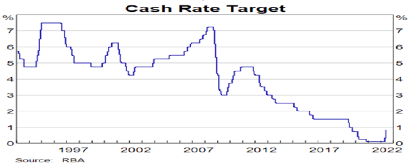
Source: RBA
Just getting started?
We’ve discussed often in these musings the (mistake?) adaptation that the US Federal Reserve made to their official monetary policy strategy back in August 2020 with the introduction of what came to be dubbed Flexible Average Inflation Targeting (FAIT). We wrote about it at the time https://convex-strategies.com/2020/09/21/risk-update-august-2020/. We often pointed to that stated willingness to let the “economy run hot” as the pivot point to the price stability issues that we see today. This simple visual aids in that point.
Figure 4: US CPI Index (white) and PCE Core Deflator Index (blue). 2% per annum Trend Line (red dash). Vertical line August 2020: The Birth of FAIT

Source: Bloomberg
Lately, we have been waiting for somebody to pose the question to Chair Powell as to his view towards the success of his introduction of FAIT as a part of their monetary policy strategy. Would he term it a success? If so, is he sticking with it? As we noted in the August 2020 Update, the launch of FAIT was met with vociferous fanfare and pronouncement from the various Fed mouthpieces. Oddly, we hear very little about it nowadays. Will they be making the equal commitment to now running the economy cold to make up for the overshoot of the last couple of years?
Donald Kohn, former Vice Chair of the Fed, gave a speech back in March on just this topic. It is well worth a read. Obviously, given his standing in that society, Mr. Kohn must come at the topic with a general acceptance that it was/is a good idea for the low inflation environment under which it was constructed. He does, however, raise the obvious complications as to how it works in the opposite environment. He puts it quite clearly.
“A crucial question is how monetary policy strategy would evolve in the framework if the problem becomes one of reducing inflation rather than getting it up to target.”
The two major central banks that continue to resist the transition away from all-time extreme monetary accommodation, in the face of multi-decade expansion of pricing measures, are the ECB and the BOJ.
As promised last month, the ECB updated their quarterly projections, giving us another chance to check in on their forecasting prowess. The projections went up as of June 9th. The revised projection for Q2 2022 HICP average monthly yoy% change was revised up to 7.5%, up rather significantly from the March 2022 projections of 5.6%. Given they already had to hand the yoy% numbers for April (7.4%) and May (8.1%), we can back out their forecast for the June yoy% number at 7%. We know now that the actual June number came in at 8.6% (8.64% to be precise). A miss, with 3 weeks remaining in a 52-week data series, of 160bp. Better than the equivalent 170bp miss on the equivalent example of the March 2022 numbers, though we wouldn’t credit them with getting any smarter.
https://www.ecb.europa.eu/pub/projections/html/ecb.projections202203_ecbstaff~44f998dfd7.en.html
We refuse to believe that Chief Economist Lane and his staff of PHDs are that incapable, so come back to the same old question – why do they incessantly try to mislead? Nobody will be surprised to see below that their longer-term projections do indeed have their price stability measure returning to their 2% target, just maybe a bit further out in the future. Why anybody assigns any credibility to these folks is beyond our understanding.
Figure 5: Eurozone HICP yoy% change (blue) vs ECB quarterly forecast through June 2022

Source: ECB, Convex Strategies
Reading either the updated projections or the policy announcement, which as expected announced the expectation of an initial 25bp at the following meeting in July (amounting to a further loosening in June, per Lagarde’s blog from late May), one gets the clear impression that the ECB would very much like to blame their inflation issues on things related to the Russia/Ukraine situation. While there is no doubt that all sorts of multi-variate reflexivity is going on across the continent, it would seem that Russia alone is not singularly the core of their problem.
https://www.ecb.europa.eu/press/pr/date/2022/html/ecb.mp220609~122666c272.en.html,
Figure 6: Eurozone PPI (white) and HICP (blue) Indices. Normalized. Vertical line (red) Feb 2022

Source: Bloomberg
The scale of the challenge reasonably jumps out when compared to the equivalent inflationary fragility in the build-up pre-GFC.
Figure 7: ECB Deposit Rate (blue), Eurozone HICP yoy% (white), Taylor Rule Estimate (yellow), Unemployment Rate (green – LHS Inverted), Projected Rate Hike (red)

Source: Bloomberg
We are unclear as to just how much that well-signalled July 21st hike in red above is going to achieve.
We will conclude our tour of June policy updates with the last man standing and still adding even further stimulus to their policy setting, our old friend BOJ Governor Kuroda. As we approached BOJ’s June policy meeting the battle was on once again as fears of an imminent adjustment to the defence of the 10yr JGB peg at 0.25% rippled through the markets. The BOJ stepped up their efforts and in an otherwise “unchanged” policy announcement did undertake formalizing some of the ad hoc technical procedural issues they put in place to maintain the peg. These were the expansion of eligible bonds for the unlimited, every day, forever Fixed Rate Operation bidding for said bonds at 0.25%. As we have discussed, they needed to deal in an immediate way with the problem of running out of bonds to buy, as well as address concerns about the implication of the divergence of the JGB future contract from the JGB cash price.
In the end, it is estimated that BOJ bought ~JPY15tn worth of bonds in June, a new record for bond buying in a single month. If/when the battle recommences, as we have suggested before, the pace of bond selling is unlikely to be linear.
https://www.japantimes.co.jp/news/2022/07/02/business/financial-markets/bank-of-japan-jgb-record/
The below chart gives a good impression of the building pressure in the far larger derivative markets as BOJ digs their heals in to hold the JGB cash peg.
Figure 8: JGB 10yr yield (white). JPY 1y10yr Forward Swap Rate (Orange). JPY 1y10y Swaption Implied Vol (purple – LHS Logged)

Source: Bloomberg
The other obvious release valves to the pressure building around their commitment to resist market determined interest rates are on-going price increases and an ever-weaker currency.
Figure 9: JGB 10yr yield (white). USD/JPY FX Rate (orange). Japan CPI yoy% (blue)

Source: Bloomberg
We have been engaged in several discussions as relates to the BOJ’s commitment to maintaining the JGB peg, what we have dubbed “the most dangerous peg in the world”. The very strong consensus within the policy world in Japan is that they are sticking with it, no matter what. We always ask the same question, “do you think it will work?” As in, do they think the continued aggressive buying of JGBs, the ongoing suppression of 10yr interest rates, will lead to their chosen inflation measure moving sustainably to 2% and above? If they say “yes”, we ask “then what are you going to do?” If they say “no”, we ask “then why do you keep doing it?”.
If they think it is going to work and buy ever more of the increasingly scarce remaining available bonds, we are going to find ourselves with Japan CPI at 3-4% and the JPY FX rate at 150.00. Is that when they will let the JGB peg go and the market deal with the adjustment of an even more significantly mispriced interest rate? If it doesn’t work, do they just keep going heedless of any acceptance of the endless failure of their extreme manipulations, and as the JPY FX rate carries on forever higher? If any of them were to be honest, they continue to pursue the policy, not because they think it will do anything of fundamental benefit, but simply because they don’t want interest rates to go up. As former-Governor Shirakawa puts it in the link at the top of this note, the longer they go, the more difficult the end-state gets.
As one of our most valued confidants put it in a private email exchange.
“The deeper question is why smart people cling on to conventional beliefs with such tenacity. The answer is not in the realm of economics.”
Last month we did a little comparison of Bank of Thailand’s 1997 effort to defend their currency peg, only to be thwarted by the uncontrollable move in their interest rates, to the Bank of Japan’s challenges today to maintain their interest rate peg and likely lose control of their currency value. (https://convex-strategies.com/2022/06/22/risk-update-may-2022/). This had set our minds on our experiences back in the heady days of the Asian Financial Crisis and led us to track down Russell Napier’s recently published tome on the topic (https://www.amazon.co.uk/Asian-Financial-Crisis-1995-98-Birth/dp/0857199145). Russell is an economic history legend. He was a strategist/economist/researcher for CLSA in HK during the ‘90s and one of the best voices forewarning and documenting the events throughout the crisis. His new book is a compilation of his actual research notes at the time with his modern-day analysis of what he got right, what he got wrong, and what is relevant to today. For those of us that lived through it, the book reads like a personal diary of the times.
It is a must read, whether you lived through it or not. That crisis was a proper crisis, very much an inflation triggered one, and can teach us a lot about what can happen after an extended period of manipulation of a key pricing and risk signal. That signal being exchange rates (thus forcing an artificial convergence of interest rates) back in those days, leading to faux volatility and correlation across all related markets and asset classes. Today, you might imagine that signal being interest rates (forcing an artificial stability of exchange rates) leading to faux volatility and correlation across all related markets and asset classes.
All this nostalgia, along with the current relevance of inflation fighting central bank rate adjustments (as we said so often over the last couple of years: “rates would be allowed to go up because central banks would decide they should”), got us thinking about the interest rate adjustments that took place to go along with the collapsing of those epic sandpiles back in ‘97/’98.
The benchmark rate in Korea, the 3mth CD Rate, peaked out at 25% and stayed between 20-25% for the better part of a year. One of our sell-side counterparties recently raised their terminal rate forecast for the Bank of Korea’s policy rate to 2.50%. We asked if they had the decimal point in the right spot.
Figure 10: Korea CPI yoy% change (grey) vs KRW 3mth CD Rate (blue)

Source: Bloomberg
Thailand, of course, was the epicentre of the subsequent series of avalanches. We can assure you that the offshore market, after the Bank of Thailand imposed capital controls in May 1997, traded implied THB interest rates through the FX swaps at significantly higher levels than BIBOR fixings were onshore.
Figure 11: Thailand CPI yoy% change (grey) vs THB 3mth BIBOR Rate

Source: Bloomberg
To get the information going back for SGD we have backed out the implied SGD interest rates from the FX swaps market for the period before the SOR benchmark existed (note, the SOR = Swap Offer Rate and is itself simply the implied interest rate backed out of the FX swap market). You can see that the wild times of the Asian Crisis years were even more than the mighty MAS could smooth out. The volatility and massive suction of USD out of the system forced the MAS to step away from their tightly managed currency band and allow a rare period of a free-floating SGD.
Figure 12: Singapore CPI yoy% change vs SGD 6mth SOR (blue) and Implied Yield from FX Swap Rate (orange)
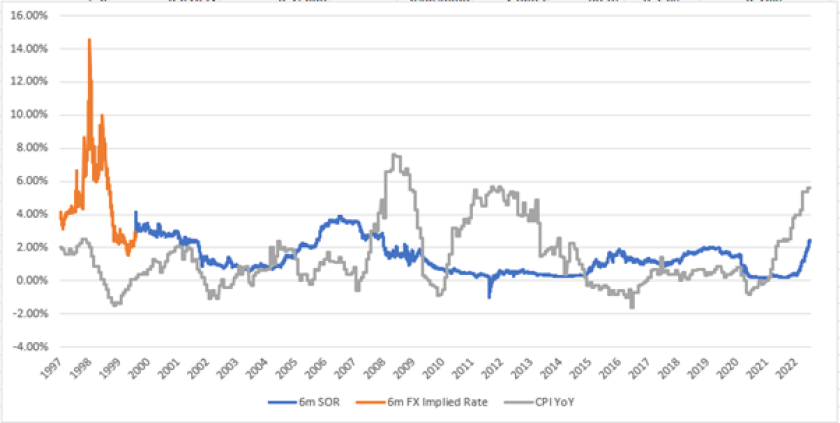
Source: Bloomberg
Looking through the range of developed markets interest rates back in that period and we can see they were much higher than today’s levels, particularly in real terms relative to their pricing measures. However, they didn’t have anywhere near the sort of spikes that were seen in the EM countries.
Figure 13: US CPI yoy% change (grey) vs USD 3mth LIBOR (blue)

Source: Bloomberg
Figure 14: UK RPI yoy% change (grey) vs GBP 3mth LIBOR (blue)

Source: Bloomberg
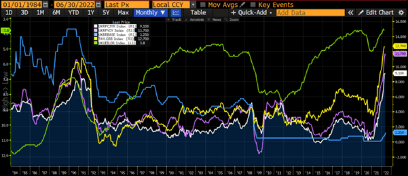
Figure 15: Australia CPI yoy% change (grey) vs AUD 3mth BBSW (blue)

Source: Bloomberg
For EUR we have again used the implied rate for the Deutschmark (DEM) from the FX swap market to construct data back before EURIBOR existed. Also, we have used the German CPI history. This chart, as always, is an eye-popper. What are they thinking?
Figure 16: German CPI yoy% change (grey) vs EUR 3mth EURIBO (blue) and DEM Implied Yield from FX Swap

Source: Bloomberg
Finally Japan, the one truly unique market. By 1997 the era of lower forever interest rates was already well underway. Maybe Japan is actually different and rates there will just stay at zero forever. Alternatively, maybe Japan is the tightest coiled spring we have ever seen.
Figure 17: Japan CPI yoy% change (grey) vs JPY 3mth TIBOR (blue)

Source: Bloomberg
We have used the picture below (Figure 18) of US Nominal GDP on several occasions. It clearly shows that, at the very least, there has been an unprecedented expansion of variance of this measure. One could make the leap that this volatility of underlying circumstances would inevitably feed through into volatility of things like interest rates, and onward across all aspects of markets. In early 2020 the spike down, driven by the response to the Covid pandemic, was on an unprecedented scale. The forced job losses as a result of pandemic policies are unlike anything ever seen.
Figure 18: US Nominal GDP yoy%, 10yr Treasury yield, Fed Funds Rate

Source: Bloomberg
Likewise, coming out the other side, the US has experienced unexpected, multi-decade extreme, spikes in inflation measures which were fuelled by extreme monetary and fiscal support.
We discussed this dynamic, and rolled out the relevance of the mathematical premise of Jensen’s Inequality, back in our December 2020 Update (https://convex-strategies.com/2021/01/22/risk-update-december-2020/). Our purpose then was to construct portfolios equally balanced to both upside and downside. Now seems like a good time to revise that analysis.
Figure 19: Jensen’s Inequality (Vol vs Var)

Source: Convex Strategies
Our starting premise was to create a portfolio that looked like the linear read lines with equal balance to upside and downside. We managed to do so with a traditional form of a Balanced Portfolio of equity (SPX) and fixed income (US Tsy) in a 10%/90% weighting. We then went through our simple “rule of thumb” Convex conversion; take the fixed income weighting (90) and split it equally between Long Volatility (45) and more equity (45), then 2x lever the Long Vol allocation, giving us a new 55%/90% convex Barbell Portfolio to get something that matches the blue function.
We built that originally to match the Jensen’s Inequality view for the recent volatile period commencing in January 2020 through to December 2020. It looked great then and looks just as good if we update it now through June 2022.
Figure 20: Jensen’s Inequality: Balanced 10%/90% vs BarBell 55%/90% Jan’20-June’22


Source: Convex Strategies, Bloomberg
Looking back even further, another relevant period to include in the comparison would be from May 2012 through December 2019, the period of peak relative outperformance of the fixed income proxy over the long vol proxy on a standalone basis, and where the opportunity cost of holding the capital in fixed income is most effectively masked. Of course, once you get into the tricky part of the racetrack, the superior convexity of the Barbell Portfolio fires up.
Figure 21: Jensen’s Inequality: Balanced 10%/90% vs Barbell 55%/90% May’12-June’22


Source: Convex Strategies, Bloomberg
If we look at it over the entire post-GFC bull market period, the comparison is still favourable.
Figure 22: Jensen’s Inequality: Balanced 10%/90% vs Barbell 55%/90% March’09-June’22


Source: Convex Strategies
Not surprisingly, extending the view back to before the GFC compares favourably as well.
Figure 23: Jensen’s Inequality: Balanced 10%/90% vs Barbell 55%/90% Jan’05-June’22


Source: Convex Strategies
In all of the above horizons, across the various views, the Barbell Portfolio displays positive convexity in the Scattergram View, positive return skew in the return distribution, and far superior compounding. True “Alpha” is to be found in improved portfolio convexity. Genuine “Alpha” is the mathematical improvement of geometrically compounded returns.
Read our Disclaimer by clicking here